Flux Balance Analysis#
Flux balance analysis (FBA) is a mathematical framework for analyzing the flow of metabolites through a metabolic network. This primer introduces the theoretical foundations of FBA, presents several practical examples, and provides a software toolbox to facilitate the necessary calculations [Orth et al., 2010].
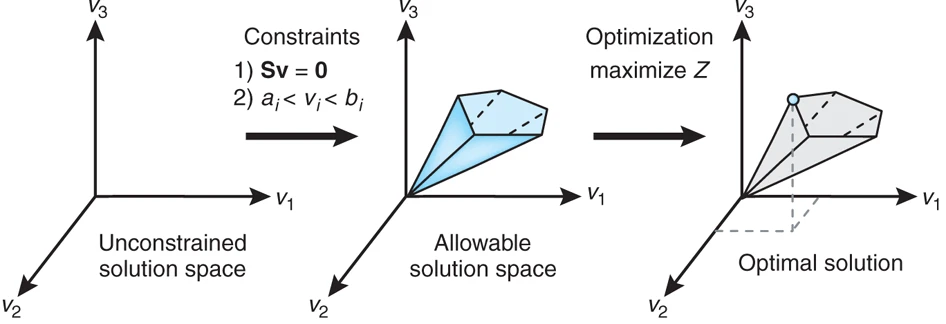
Fig. 3 The conceptual basis of constraint-based modeling.#
Environment Setup#
For performing comprehensive constraint-based metabolic network analyses, several specialized software tools are required. In this section, we will install and configure two key components: the COBRA Toolbox and Gurobi. The COBRA Toolbox is a MATLAB-based software suite specifically designed for the analysis of genome-scale biochemical networks, while Gurobi is a state-of-the-art optimization solver that provides a MATLAB interface for executing linear and mixed-integer linear programming tasks.
The Constraint-Based Reconstruction and Analysis (COBRA) Toolbox is widely recognized for its robust framework, enabling quantitative predictions of cellular and multicellular biochemical networks under various constraints. It implements an extensive range of methodologies, from fundamental reconstruction and model generation techniques to advanced, unbiased approaches for model-driven analysis. By integrating the COBRA Toolbox into a MATLAB environment, researchers gain access to a versatile platform for modeling, analyzing, and predicting diverse metabolic phenotypes at the genome scale [Heirendt et al., 2019].
Gurobi is a state-of-the-art mathematical optimization solver, widely recognized for its exceptional performance and reliability in solving a broad spectrum of linear, integer, and mixed-integer linear programming problems. Its advanced algorithms, parallelized computations, and extensive parameter tuning options make it one of the most efficient and user-friendly optimization tools available [Gurobi 12.0 Documentation, 2024]. By providing a robust MATLAB interface, Gurobi seamlessly integrates with the COBRA Toolbox and other computational frameworks, thereby streamlining model-driven analysis and facilitating rapid, large-scale solution of complex optimization problems.
FBA model construction#
Here, we present a very simple example of a Flux Balance Analysis (FBA) study. As shown in the Fig. 4, this is not an actual cell, but rather a hypothetical one used for illustrative purposes. We refer to the interior of the cell as the “intracellular”, and the environment outside the cell as the “extracellular”. In this simplified scenario, the cell consumes a substrate from the side labeled \(b_{1}\), where \(b_{1}\) represents the rate of consumption. Once this substrate crosses the membrane, an action known as “uptake,” it is referred to as metabolite \(A\) within the cell.
Within the cell, there are several reactions involving metabolites \(A\), \(B\), and \(C\). The reactions from \(A\) to \(B\) and from \(C\) to \(B\) are irreversible, while the reaction between \(A\) and \(C\) is reversible. Additionally, the cell can secrete metabolite \(B\) back into the extracellular environment, and similarly, it can secrete metabolite \(C\). Thus, we have one uptake process and two secretion processes.
Conceptually, this is essentially a set of kinetic or, more specifically, mass balance equations. In an actual cell, there would be hundreds of such exchanges and reactions, and instead of just three metabolites, a large-scale metabolic model might include thousands. For example, in the iMM904 metabolic reconstruction, there are approximately 4,000 metabolites. A real model is typically much larger and more complex, but this basic scenario helps convey the general idea of how FBA works.
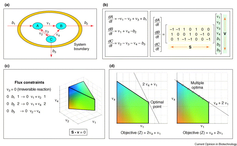
Fig. 4 Methodology for flux balance analysis [Kauffman et al., 2003].#
Once we have set up the basic system, we can write mass-balance equations for each metabolite. Let us denote the concentrations of metabolites \(A\), \(B\), and \(C\) by \([A]\), \([B]\), and \([C]\), respectively. Their time derivatives (accumulation rates) are given by sums of all reactions that either produce or consume these metabolites.
As an example, consider the balance for metabolite \(A\). Its net rate of change is given by
Here:
\(b_{1}\) and \(v_{3}\) represent the reactions producing \(A\), hence the positive sign.
\(v_{1}\) and \(v_{2}\) are two reactions consuming \(A\), hence the negative sign.
We can perform the same process for metabolites B and C as well. After writing these mass-balance equations, we can assemble them into a stoichiometric matrix, often denoted by \(S\). Then the mass balances for all metabolites can be written in compact form as (2), as also depicted in the right part of Fig. 4b.
Typically, the stoichiometric matrix and flux vector are denoated as \(S\) and \(v\), respectively, with the goal of determining the flux distribution under known constraints. The flux vector includes all reaction rates, including uptake and secretion fluxes as well as internal metabolic fluxes. In a practical scenario, we specify the stoichiometric matrix for the organism of interest. Each organism has its own unique matrix, reflecting its metabolic network and available metabolites. We might specify the uptake flux (e.g., \(b_{1}\)) and then attempt to solve for all unknown fluxes, including the internal fluxes and secretion fluxes.
To simplify the problem, we often assume a steady-state condition, setting all time derivatives to zero. Additionally, certain reactions may be excluded from consideration; for example, assuming \(V_{3}=0\), effectively making the A-to-C pathway one-way (irreversible). After applying these simplifications, we might end up with a system that has three equations but five unknowns. Because there are more unknowns than equations, the system is underdetermined and cannot be solved uniquely.
To address this issue, we introduce an optimization objective. In FBA, a common objective is to assume that the cell optimizes its metabolic fluxes to maximize growth rate. In simpler conceptual models, we might choose a different arbitrary objective, but the principle remains the same: we impose an additional criterion to select a unique solution from the set of all feasible solutions, as demonstrated by Fig. 4c,d.
Geometrically, if we consider the feasible set of flux distributions as a region in flux space, the objective function defines contours of constant objective value. We then seek the point in the feasible region that yields the maximum value of the objective. The mathematical formulation, with a linear objective and linear constraints derived from the stoichiometric equations and flux bounds, takes the form of a linear programming (LP) problem.
A general linear program looks like this:
Maximize (or minimize) a linear objective function:
where \(\mathcal{c}\) is a vector of known coefficients and \(x\) represents the fluxes we are trying to determine.
Subject to:
A set of linear constraints, which can include equalities or inequalities. In FBA, the stoichiometric constraints are often equalities, for example:
Bounds on the variables (fluxes):
Solving such a system requires specialized linear programming software, such as Gurobi, which is commonly used for FBA problems. By posing the FBA problem as a linear program, we can find the flux distribution that optimizes the chosen objective, thereby providing insights into the cell’s metabolic strategies.
Genome-Scale Metabolic Model#
Saccharomyces cerevisiae, a widely used model organism in eukaryotic studies, has long been employed to investigate genetic interactions, to serve as a platform for constructing cell factories that produce high-value compounds, and to deepen our understanding of eukaryotic metabolism. Over the past two decades, the genome-scale metabolic models (GEMs) of S. cerevisiae have undergone continuous refinement and enhancement, culminating in a series of models that includes Yeast9 [Zhang et al., 2024], Yeast8 [Lu et al., 2019], Yeast7 [Aung et al., 2013], Yeast5 [Heavner et al., 2012], Yeast4 [Dobson et al., 2010], Yeast1 [Herrgård et al., 2008], iMM904 [Mo et al., 2009], iIN800 [Nookaew et al., 2008], iLL672 [Kuepfer et al., 2005], and iND750 [Duarte et al., 2004]. This progression builds on the foundational first-generation model, iFF708, published in 2003 [Förster et al., 2003].
Within this chapter, we will apply a classic Yeast GEM model, iMM904, available through the BiGG database. The Biochemical, Genetic, and Genomic knowledgebase (BiGG Models) is an open-source, community-driven resource providing standardized, genome-scale metabolic network models [Norsigian et al., 2020]. It offers a comprehensive platform for researchers, students, and bioinformatics professionals to access high-quality reconstructions spanning a wide range of organisms. As of version 1.6, updated in 2019, BiGG Models features 108 published models. For more detailed information, please visit http://bigg.ucsd.edu/models.
Example: FBA with iND750 Yeast Model#
You are given the iND750 genome-scale metabolic model for S. cerevisiae. In a laboratory setting, you want to grow this yeast under the following conditions:
Carbon Source (Glucose): 20 g/L
Oxygen (Gas): 2 mmol/L
Use Flux Balance Analysis (FBA) to determine the yeast’s predicted biomass concentration (or specific growth rate) under these constraints.